Complex integration. Complex and real line integrals, Properties. Green�s theorem in the plane, Cauchy�s integral theorem, Morera�s theorem, indefinite integral, simply and multiply-connected regions, Jordan curve

SolitaryRoad.com

Website owner:  James Miller

[ Home ] [ Up ] [ Info ] [ Mail ]

Complex integration. Complex and real line integrals, Green’s theorem in the plane, Cauchy’s integral theorem, Morera’s theorem, indefinite integral, simply and multiply-connected regions, Jordan curve

An integral that is evaluated along a curve is called a line integral. Such integrals can be defined in terms of limits of sums as are the integrals of elementary calculus.

Def. Complex line integral. Let C be a rectifiable curve (i.e. a curve of finite length) joining points a and b in the complex plane and let f(z) be a complex-valued function of a complex variable z, continuous at all points on C. Subdivide C into n segments by means of points a = z₀, z₁, ... , z_n = b selected arbitrarily along the curve. On each segment joining z_k-1to z_kchoose a point ξ _k . Form the sum

Let Δ be the length of the longest chord Δz_k. Let the number of subdivisions n approach infinity in such a way that the length of the longest chord approaches zero. The sum S_n will then approach a limit which does not depend on the mode of subdivision and is called the line integral of f(z) from a to b along the curve:

Theorem 1. If F is a function such that dF(z)/dz = f(z) at each point of C, then

Real line integrals. There are different types of real line integrals. The most common type is

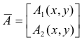
where is a vector point function

defined over some region R of the plane, is a position vector

to point P on a curve C within R, the product is the dot product and the integral is evaluated along C. is given by

and

can be written as

The line integral from point A to point B on C

can be written equivalently as

where T is the unit tangent to the curve and s is arc length along C. If represents a force field, the integral represents the amount of work done in moving an object along the curve from point A to point B.

If arc AB over which the integral is to be evaluated is smooth and given by the parametric equations

where t₁ t t₂ , the value of 3) is given by

Theorem 2. Consider the real line integral

If P(x, y)dx + Q(x, y)dy, or more concisely, Pdx + Qdy, is an exact differential i.e. if

there is a function Φ(x, y) such that dΦ = Pdx + Qdy and the line integral is equal to the change of Φ(x, y) along the curve from point A to point B. Moreover, if ∂P / ∂y = ∂Q /∂x everywhere in a simply connected region, the value of the line integral between two points of the region does not depend on the path of integration.

Connection between real and complex line integrals. Real and complex line integrals are connected by the following theorem.

Theorem 3. If f(z) = u(x, y) + i v(x, y) = u + iv, the complex integral 1) can be expressed in terms of real line integrals as

Because of this relationship 5) is sometimes taken as a definition of a complex line integral.

Note that if the Cauchy-Riemann equations

are satisfied, both integrands “u dx - v dy” and “v dx - u dy” in the right member of 5) are exact differentials.

Intuitive interpretation of complex integral. What kind of intuitive, physical interpretation can one give to the complex integral? From 5) and 3) we see that

where

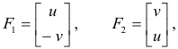
T is the unit tangent to the curve and s is arc length along the curve. The real and imaginary parts of 6) can be viewed as representing work done in the two force fields F₁ and F₂.

Properties of line integrals

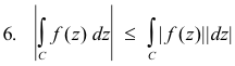
If f(z) and g(z) are integrable along curve C, then

where |f(z)| M ( i.e. M is an upper bound of |f(z)| on C) and L is the length of C.

Proof

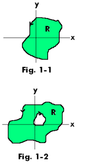
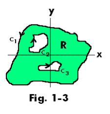
Def. Simply-connected region. A region R is said to be simply-connected if any simple closed curve which lies in R can be shrunk to a point without leaving R. A region R which is not simply-connected is said to be multiply-connected. The region shown in Fig. 1-1 is simply-connected. The regions shown in Figures 1-2 and 1-3 are multiply-connected.

Def. Jordan curve. Any continuous closed curve that does not intersect itself. Its length may be finite or infinite.

An intuitively obvious but very difficult to prove theorem follows:

Jordan Curve Theorem. A Jordan curve divides the plane into two regions having the curve as a common boundary.

The region that is bounded is called the interior and the other region is called the exterior.

Convention regarding traversal of a closed path. The boundary of a region is said to be traversed in the positive sense or direction if an observer traveling in this direction has the region to the left. Note the arrows in Figures 1-1, 1-2 and 1-3 and how those on the inner boundaries in the multiply-connected regions are pointed in the opposite direction from those on the outer boundary.

The notation

is used to denote integration of f(z) around the boundary C of a region in the positive sense. A full trip around the entire boundary is assumed. C denotes the aggregate of curves forming the boundary. In the multiply-connected region shown in Fig. 1-3 the boundary includes the entirety of curves c₁, c₂ and c₃. This integral is called a contour integral.

Green’s Theorem in the plane. Let P(x, y) and Q(x, y) be continuous and have continuous partial derivatives in a closed region R, either simply or multiply-connected, and on its boundary C. Then

Proof

Complex form of Green’s Theorem. Let F(z, ) be continuous and have continuous partial derivatives in a closed region R, either simply or multiply-connected, and on its boundary C. Then

where dA represents the element of area dxdy and z and are complex conjugate coordinates z = x + iy and = x - iy.

Proof

Cauchy’s integral theorem. Let a function f(z) be analytic within and on the boundary of a region R, either simply or multiply-connected, and let C be the entire boundary of R. Then

See Fig. 1-3 above.

Syn. Cauchy’s theorem, Cauchy-Goursat theorem

Proof

This theorem was first proved with the added condition that f '(z) be continuous in R and then Goursat gave a proof that removed this condition.

The following theorem is an immediate consequence of Cauchy’s integral theorem.

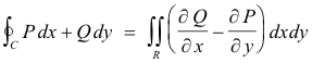
Theorem 4. Let a function f(z) be analytic in a simply-connected region R and let C be a closed (not necessarily simple) curve in R. Then

See Fig. 2.

Proof

Another immediate consequence of Cauchy’s integral theorem is the following theorem.

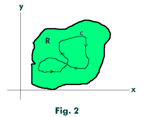
Theorem 5. If f(x) is analytic in and on the boundary of the region R between two simple closed curves C₁ and C₂ then

where C₁ and C₂ are both traversed in the positive sense relative to their interiors (counterclockwise). See Fig. 3.

Proof

Since there may be points in the interior of C₂ where f(z) is not analytic, we cannot say that either of these integrals is zero. However, they do have the same value. Theorem 5 leads us to the extremely important principle of the deformation of contours:

Principle of the deformation of contours. The line integral of an analytic function around any closed curve C₁ is equal to the line integral of the same function around any other closed curve C₂ into which C₁ can be continuously deformed without passing through a point where f(z) is nonanalytic.

Theorem 5 can be generalized in the following theorem.

Theorem 6. Let f(z) be analytic both in a region R bounded by the non-overlapping simple closed curves C, C_1, C₂, ..., C_n, where C_1, C₂, ..., C_n are inside curve C (see Fig. 4), and on the curves themselves. Then

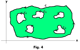
where C₁, C₂, ... , C_n are traversed in the positive sense relative to their interiors (counterclockwise).

Morera’s Theorem. Let f(z) be continuous in a simply-connected region R and suppose that

around every simple closed curve C in R. Then f(z) is analytic in R.

This theorem, often called the converse of Cauchy’s theorem, is also valid for multiply-connected regions.

Def. Indefinite integral. If f(z) and F(z) are analytic in a region R and such that dF(z)/dz = f(z), then F(z) is called an indefinite integral of f(z) and denoted by

Syn. Anti-derivative, primitive

Theorem 7. Let f(z) be analytic in a simply-connected region R. If a and b are any two points in R, then

is independent of the path in R joining a and b.

Proof

Theorem 8. Let f(z) be analytic in a simply-connected region R. If a and z are any two points in R and

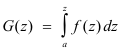
then G(z) is analytic in R and G'(z) = f(z).

Theorem 9. Let f(z) be analytic in a simply-connected region R. If a and b are any two points in R and F'(z) = f(z), then

Example.

References

Mathematics, Its Content, Methods and Meaning

James and James. Mathematics Dictionary

Spiegel. Complex Variables (Schaum)

Wylie. Advanced Engineering Mathematics

Hauser. Complex Variables with Physical Applications.