Chi-square test. Contingency tables. Yates’ correction. Coefficient of Contingency.

SolitaryRoad.com

Website owner:  James Miller

[ Home ] [ Up ] [ Info ] [ Mail ]

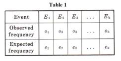
Observed and theoretical frequencies. Suppose that in an experiment a set of possible events E₁, E₂, .... , E_k are observed to occur with frequencies o₁, o₂, o₃, .... , o_k, called observed frequencies, and that according to probability rules they are expected to occur with frequencies e₁, e₂, e₃, .... , e_k, called expected or theoretical frequencies. See Table 1. We often wish to know whether observed frequencies differ significantly from expected frequencies. We now treat that problem.

A measure of the discrepancy existing between observed and expected frequencies is supplied by the statistic χ² (read chi-square) given by

where if the total frequency is n, then

2) ∑o_j = ∑e_j = n .

It can be shown that 1) is equivalent to

Proof

If χ² = 0, observed and theoretical frequencies agree exactly. If χ² > 0, they do not agree exactly. The larger the value of χ², the greater is the discrepancy between observed and expected frequencies.

The sampling distribution of χ² is approximated very closely by the chi-square distribution

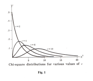
if expected frequencies are at least equal to 5, the approximation improving for larger values. See Fig. 1.

The number of degrees of freedom ν is given by

(a) ν = k - 1 if expected frequencies can be computed without having to estimate population parameters from sample statistics. Note that we subtract 1 from k because of the constraint condition 2) which states that if we know k - 1 of the expected frequencies the remaining frequency can be determined.

(b) ν = k - 1 - m if the expected frequencies can be computed only by estimating m population parameters from sample statistics.

Significance tests. In practice, expected frequencies are computed on the basis of a hypothesis H₀. Using the null hypothesis we compte the expected frequencies and then the value of χ². If the value of χ² is greater than some critical value n (such as or which are the critical values at the .05 and .01 significance levels respectively) we conclude that the observed frequencies differ significantly from expected frequencies and reject H₀. Otherwise, we accept H₀(or at least not reject it).

This procedure is called the chi-square test of hypothesis or significance.

The chi-square test for goodness of fit. The chi-square test can be used to determine how well theoretical distributions, such as the normal, binomial, etc., fit empirical distributions (i.e. those obtained from sample data).

Contingency tables. Table 1 above, in which observed frequencies occupy a single row, is called a one-way classification table. Since the number of columns is k, this is also called a 1 × k (read “1 by k”) table. By extending these ideas we arrive at two-way classification tables or h × k tables in which the observed frequencies occupy h rows and k columns. Such tables are often called contingency tables.

Corresponding to each frequency in an h × k contingency table, there is an expected or theoretical frequency which is computed subject to some hypothesis according to rules of probability. These frequencies which occupy the cells of a contingency table are called cell frequencies. The total frequency in each row or each column is called the marginal frequency.

To investigate agreement between observed and expected frequencies, we compte the statistic

where the sum is taken over all cells in the contingency table, the symbols o_j and e_j representing respectively the observed and expected frequencies in the jth cell. This sum which is analogous to 1) contains hk terms. The sum of all observed frequencies is denoted by n and is equal to the sum of all expected frequencies.

As before, the statistic 5) has a sampling distribution given very closely by 4), provided expected frequencies are not too small. The number of degrees of freedom ν of this chi-square distribution is given for h > 1, k > 1 by

(a) ν = (h -1)(k - 1) if the expected frequencies can be computed without having to estimate population parameters from sample statistics.

(b) ν = (h -1)(k - 1) - m if the expected frequencies can be computed only by estimating population parameters from sample statistics.

Significance tests for h×k tables are similar to those for 1×k tables. Expected frequencies are found subject to a particular hypothesis H₀. A hypothesis commonly assumed is that the two classifications are independent of each other.

Contingency tables can be extended to higher dimensions. Thus, for example, we can have h×k×l tables where 3 classifications are present.

Yates’ correction for continuity. When results for continuous distributions are applied to discrete data, certain corrections for continuity can be made. The correction consists in rewriting 1) as

and is usually referred to as Yates’ correction. An analogous modification of 5) also exists.

In general, the correction is made only when the number of degrees of freedom is ν = 1. For large samples this yields practically the same results as the uncorrected χ², but difficulties can arise near critical values. For small samples where each expected frequency is between 5 and 10, it is perhaps best to compare both the corrected and uncorrected values of χ².

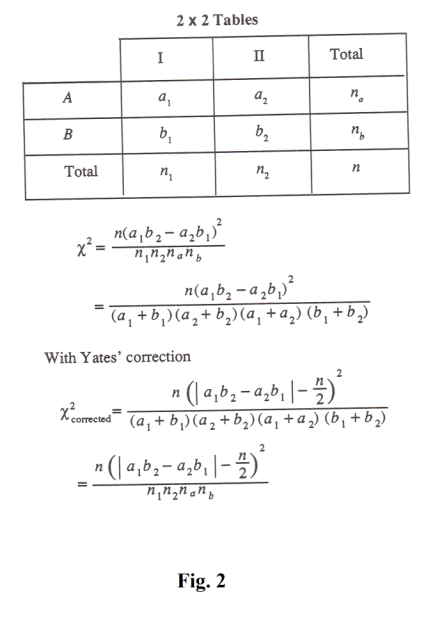
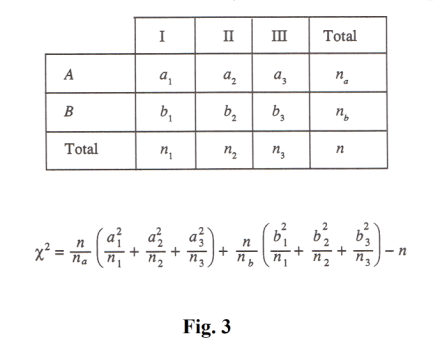
Simple formulas for computing χ². Simple formulas for computing χ² which involve only the observed frequencies can be derived. See Fig. 2 and Fig. 3 for the cases of 2×2 and 2×3 tables.

Coefficient of Contingency. A measure

of the degree of relationship, association or dependence of the classifications in a contingency table is given by

which is called the coefficient of contingency. The larger the value of C, the greater is the degree of association. The number of rows and columns in the contingency table determines the maximum value of C, which is never greater than one. If the number of rows and columns of a contingency table is equal to k, the maximum value of C is given by .

Correlation of attributes. Because classifications in a contingency table often describe characteristics of individuals or objects, they are often referred to as attributes and the degree of dependence, association or relationship is called correlation of attributes. For k × k tables we define

as the correlation coefficient between attributes or classifications. This coefficient lies between 0 and 1. For 2 × 2 tables in which k = 2, the correlation is often called tetrachoric correlation.

Additive property of χ². Suppose the results of repeated experiments yield sample values of χ² given by with ν₁, ν₂, ν₃, ... degrees of freedom respectively. Then the result of all these experiments can be considered equivalent to a χ² value given by with ν₁ + ν₂+ ν₃ + .... degrees of freedom.

Portions excerpted from Murray R. Spiegel. Statistics. Schaum.

References

Murray R Spiegel. Statistics (Schaum Publishing Co.)