Website owner: James Miller
Equations of the first order and higher degree, Clairaut’s equation. Singular solutions and extraneous loci. Discriminant of a differential equation. p-discriminant, c-discriminant.
General first order equation of degree n. The general first order equation of degree n is an equation of the form
1) a0(x, y)(y')n + a1(x, y)(y')n -1 + .... + an-1(x, y)y' + an(x, y) = 0
or, equivalently,
2) a0(x, y) pn + a1(x, y)pn -1 + .... + an-1(x, y)p + an(x, y) = 0
where in 2) we have used the usual convention of denoting y' by the letter p.
Examples. The following equations are of the first order and varying degrees:
xy (y')2 + (x2 + xy + y2)y' + x2 + xy = 0 degree 2
(x2 + 1)(y')4 + (x + 3 y)(y')2 + 2x2 + y = 0 degree 4
(xy + 2)(y')3 + (y')2 + 5x2 = 0 degree 3
Such equations can sometimes be solved by one or more of the following methods. In each case the problem is reduced to that of solving one or more equations of the first order and first degree.
Methods of solution
I Equations solvable for p. Here the left member of 2), viewed as a polynomial in p, can be resolved into n linear real factors i.e. 2) can be put into the form
(p - F1)(p - F2) ...... (p - Fn) = 0
where the F’s are functions of x and y.
Procedure. Factor into n linear real factors, set each factor equal to zero and solve the resulting n differential equations of the first order and first degree
![]()
to obtain
3) f1(x, y, C) = 0, f2(x, y, C) = 0, .......... , fn(x, y, C) = 0
The primitive of 2) is the product
f1(x, y, C) · f1(x, y, C) · .................. · f1(x, y, C) = 0
of the n solutions 3).
Example. Solve
xy (y')2 + (x2 + xy + y2)y' + x2 + xy = 0
Solution. In terms of p this equation is
xy p2 + (x2 + xy + y2)p + x2 + xy = 0
and factored as
(xp + x + y)(yp + x) = 0
The solutions of the component equations
![]()
are respectively
2xy + x2 - C = 0 and x2 + y2 - C = 0
The primitive is (2xy + x2 - C )(x2 + y2 - C) = 0
II Equations solvable for y, i.e. equations expressible as y = f(x, p).
Procedure.
1. Differentiate y = f(x, p) with respect to x to obtain
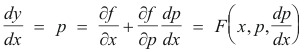
an equation of the first order and first degree.
2. Solve p = F(x, p, dp/dx) to obtain φ(x, p, C) = 0.
3. Obtain the primitive by eliminating p between y = f(x, p) and φ(x, p, C) = 0, when possible, or express x and y separately as functions of the parameter p.
Example. Solve
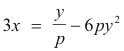
1) 16x2 + 2p2y - p3x = 0
Solution. We can rewrite the equation as
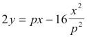
Differentiating with respect to x we get
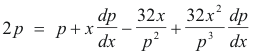
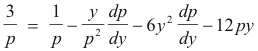
Clearing of fractions and combining we have
![]()
or
![]()
This equation is satisfied when p3 + 32x = 0 or p - x(dp/dx) = 0. From the later we obtain

Integrating we get
ln p = ln x + ln K = ln Kx
Taking exponentials we get
3) p = Kx
Substituting 3) into 1) we get
16x2 + 2K2x2y - K3 x4 = 0
or, replacing K by 2C,
2 + C2y - C3x2 = 0
which is the primitive.
We will not consider the factor p3 + 32x of 2) here because it does not contain the derivative dp/dx. Use of the factor will yield a singular solution, a topic that we will treat shortly.
III Equations solvable for x, i.e. equations expressible as x = f(y, p).
Procedure.
1. Differentiate x = f(y, p) with respect to y to obtain
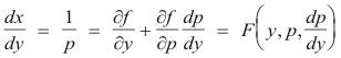
an equation of the first order and first degree.
2. Solve 1/p = F(y, p, dp/dy) to obtain φ(y, p, C) = 0.
3. Obtain the primitive by eliminating p between x = f(y, p) and φ(y, p, C) = 0, when possible, or express x and y separately as functions of the parameter p.
Example. Solve
1) y = 3px + 6p2y2
Solution.
Solving 1) for x we obtain
Differentiating with respect to y we obtain
Clearing of fractions we obtain
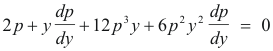
or
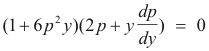
Setting the second factor equal to zero gives
Integrating we get
2 ln y = - ln p + ln C
which yields
py2 = C
or, equivalently,
2) p = C/y2
Substituting 2) into 1) gives the primitive
y3 = 3Cx + 6C2
IV Clairaut’s equation. The differential equation
y = px + f(p)
is called Clairaut’s equation. Its primitive is
y = Cx + f(C)
and is obtained simply by replacing p by C in the given equation.
Example. Solve
![]()
Solution. The primitive is
![]()
Source: Ayres. Differential Equations (Schaum). Chap 9
Singular solutions and extraneous loci
Singular solutions. In addition to the general solution a differential equation may also have a singular solution. A singular solution is a solution not obtainable by assigning particular values to the arbitrary constants of the general solution. It is the equation of an envelope of the family of curves represented by the general solution. This envelope satisfies the differential equation because at every one of its points its slope and the coordinates of the point are the same as those of some member of the family of curves representing the general solution.
James/James. Mathematics Dictionary.
Def. Discriminant of a differential equation. p-discriminant, c-discriminant. For a differential equation of type f(x, y, p) = 0, where p = dy/dx, the p-discriminant is the result of eliminating p between the equations f(x, y, p) = 0 and ∂f(x, y, p)/∂p = 0. If the solution of the differential equation is
u(x, y, c) = 0
the c-discriminant is the result of eliminating c between the equations u(x, y, c) = 0 and ∂u(x, y, c)∂c = 0. The curve whose equation is obtained by setting the p-discriminant equal to zero contains all envelopes of solutions, but also may contain a cusp locus, a tac-locus, or a particular solution (in general, the equation of the tac-locus will be squared and the equation of the particular solution will be cubed). The curve whose equation is obtained by setting the c-discriminant equal to zero contains all envelopes of solutions, but also may contain a cusp locus, a node locus, or a particular solution (in general, the equation of the node-locus will be squared and the equation of the particular solution will be cubed). In general, the cusp locus, node locus and tac-locus are not solutions of the differential equation.
Example. The differential equation (dx/dy)2(2 - 3y)2 = 4(1 - y) has the general solution (x - c)2 = y2(1 - y) and the p-discriminant and c-discriminant equations are, respectively,
(2 - 3y)2(1 - y) = 0 and y2(1 - y) = 0 .
The line 1 - y = 0 is an envelope; 2 - 3y = 0 is a tac-locus; y = 0 is a node locus.
James/James. Mathematics Dictionary.
Let us now consider a concrete example of an equation containing a singular solution.. The differential equation
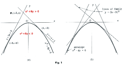
1) y = px + 2p2
has as its general solution the family of straight lines
2) y = Cx + 2C2.
In addition to this general solution it also has the singular solution
3) x2 + 8y = 0
which is a parabola. See Fig. 1.
Typical lines of the general solution are shown in Fig. 1 (b). There is a single line for each value of the arbitrary constant C and each line is tangent to the singular solution i.e. the parabola x2 + 8y = 0 . We see that the singular solution corresponds to an envelope of that family of curves represented by the general solution.
In the region above the parabola x2 + 8y > 0 and in the region below the parabola x2 + 8y < 0. At each point P:(x, y) in the region above the parabola equation 1) yields a set of two distinct directions (or slopes) p1 and p2 and through P passes two distinct lines of the general solution y = Cx + 2C2 , one with the slope p1 and the other with the slope p2. For example, consider the point P:(-2, 4). If we substitute the coordinates (-2, 4) into 1) we get 4 = -2p + 2p2 , which when solved for p, gives the solutions p1 = 2 and p2 = -1. Using the point-slope formula for straight lines we compute the equations of the general solution lines passing through P with slopes p1 and p2 as y = 2x + 8 and y = -x + 2. See Fig. 1 (a). Thus passing through each point P above the parabola, there are two straight lines of the general solution, both tangent to the parabola, as shown in Fig. 1 (a).
Now let us substitute the coordinates pf point P:(-2, 4) into equation 2), the equation of the general solution. We get 4 = -2C + 2C2, which when solved for C gives the solutions C1 = 2 and C2 = -1. These two values of C, when plugged into equation 2), give the two equations y = 2x + 8 and y = -x + 2 that pass through point P.
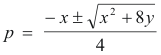
Let us now consider what happens when we move point P down towards the parabola. As we move it down the lines adjust, remaining tangent to the parabola. What happens when point P touches the parabola? The two lines become a single line tangent to the parabola. In the situation when P lies on the parabola the two slopes p1 and p2 obtained from equation 1) are equal i.e. equation 1) has multiple roots (two equal roots). If we solve equation 1) for p using the quadratic formula we get
In the situation where P lies on the parabola the discriminant x2 + 8y inside the radical sign becomes zero and the formula yields multiple roots i.e. two equal roots.
Points for which x2 + 8y < 0 yield imaginary roots for p in equation 1) and for C in equation 2).
Def. p-equation. The differential equation, expressed in terms of the letter p. In our example, equation 1) is the p-equation.
Def. C-equation. The general solution (primitive) of the differential equation. In our example, equation 2) is the C-equation.
Singular solutions and multiple roots. The singular solutions of a differential equation are found by expressing the conditions
a) that the p-equation have multiple roots
b) that the C-equation have multiple roots
Theorem 1. An equation f(x) = 0 will have multiple roots if and only if its discriminant vanishes.
Theorem 2. The discriminant of an equation f(x) = 0 can be obtained by eliminating x between f(x) = 0 and f '(x) = 0.
Discriminants of some special equations
Equation Discriminant
ax2 + bx + c = 0 b2 - ac
ax3 + bx2 + cx + d = 0 b2c2 + 18abcd - 4ac3 - 4b3d - 27a2d2
From Theorem 2, we see that if we are dealing with a p-equation the discriminant can be obtained by eliminating p between f(p) = 0 and df (p)/dp = 0. I f we are dealing with a C-equation the discriminant can be obtained by eliminating C between f(C) = 0 and df (C)/dC = 0.
Types of equations having singular solutions. In general, an equation of the first order does not have singular solutions. An equation of the first degree cannot have singular solutions. In addition, an equation f(x, y, p) = 0 cannot have singular solutions if f(x, y, p) can be resolved into factors which are linear in p and rational in x and y.
Theorem 3. Let q(x, y) = 0 be a singular solution of the differential equation f(x, y, p) = 0 and let g(x, y, C) = 0 be the general solution. Then q(x, y) is a factor of both discriminants (p-discriminant and C-discriminant). Each discriminant may, however, have other factors which give rise to other loci associated with the general solution. The p-discriminant may have factors corresponding to a tac-locus, cusp locus or a particular solution. The C-discriminant may have factors corresponding to a cusp locus, node locus or a particular solution. Tac-loci, cusp loci and node loci are extraneous i.e. they do not satisfy the differential equation.
References
1. James/James. Mathematics Dictionary.
2. Frank Ayres. Differential Equations (Schaum).
Jesus Christ and His Teachings
Way of enlightenment, wisdom, and understanding
America, a corrupt, depraved, shameless country
On integrity and the lack of it
The test of a person's Christianity is what he is
Ninety five percent of the problems that most people have come from personal foolishness
Liberalism, socialism and the modern welfare state
The desire to harm, a motivation for conduct
On Self-sufficient Country Living, Homesteading
Topically Arranged Proverbs, Precepts, Quotations. Common Sayings. Poor Richard's Almanac.
Theory on the Formation of Character
People are like radio tuners --- they pick out and listen to one wavelength and ignore the rest
Cause of Character Traits --- According to Aristotle
We are what we eat --- living under the discipline of a diet
Avoiding problems and trouble in life
Role of habit in formation of character
Personal attributes of the true Christian
What determines a person's character?
Love of God and love of virtue are closely united
Intellectual disparities among people and the power in good habits
Tools of Satan. Tactics and Tricks used by the Devil.
The Natural Way -- The Unnatural Way
Wisdom, Reason and Virtue are closely related
Knowledge is one thing, wisdom is another
My views on Christianity in America
The most important thing in life is understanding
We are all examples --- for good or for bad
Television --- spiritual poison
The Prime Mover that decides "What We Are"
Where do our outlooks, attitudes and values come from?
Sin is serious business. The punishment for it is real. Hell is real.
Self-imposed discipline and regimentation
Achieving happiness in life --- a matter of the right strategies
Self-control, self-restraint, self-discipline basic to so much in life