Vector integration, line integrals, surface integrals, volume integrals

SolitaryRoad.com

Website owner:  James Miller

[ Home ] [ Up ] [ Info ] [ Mail ]

VECTOR INTEGRATION, LINE INTEGRALS, SURFACE INTEGRALS, VOLUME INTEGRALS

Integration of vector functions. In ordinary calculus we compute integrals of real functions of a real variable; that is, we compute integrals of functions of the type

y = f(x)

where x and y are real numbers.

In vector analysis we compute integrals of vector functions of a real variable; that is we compute integrals of functions of the type

f(t) = f₁(t) i + f₂(t) j + f₃(t) k

or equivalently,

where f₁(t), f₂(t), and f₃(t) are real functions of the real variable t.

Indefinite integral. Let f(t) = f₁(t) i + f₂(t) j + f₃(t) k be a vector depending on a single real variable t, where f₁(t), f₂(t), and f₃(t) are assumed to be continuous in a specified interval. By definition, the indefinite integral of f(t), if it exists, is given as

or equivalently,

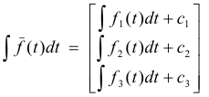
where c₁, c₂ and c₃ are constants. It exists if and only if there exists some vector F(t) such that

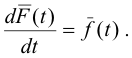
It will exist if the terms on the right side of 1) are integrable.

The indefinite integral can also be defined as a limit of a sum in a manner analogous to that of elementary integral calculus.

Definite integral. If the integral of the function f(t) exists, let it be denoted by F(t) + c. Then the definite integral of f(t) between the limits t = a and t = b is given by

Problem. The acceleration of a particle at any time t 0 is given by

a = dv/dt = 12 cos 2t i - 8 sin 2t j + 16 t k .

Find the velocity at time t, if v = 0 at t = 0.

Solution.

dv = 12 cos 2t i dt - 8 sin 2t j dt + 16 t k dt

Integrating

= 6 sin 2t i + 4 cos 2t j + 8t² k + c₁

Putting v = 0 when t = 0,

0 = 0i + 4j + 0k + c₁ .

Thus

c₁ = -4j

and

v = 6 sin 2t i + (4 cos 2t - 4) j + 8t² k

Line integrals.

*******************

There are different types of line integrals. In general, any integral that is evaluated along a curve is called a line integral. The curves are usually given in parametric form such as

x = x(t)

y = y(t)

z = z(t) .

Such integrals can be defined in terms of limits of sums as are the integrals of elementary calculus.

Types of line integrals.

1] ∫_c f(x,y,z) dR

where f(x,y,z) is a scalar point function of x, y, z and R is a radius vector R(t) = x(t) i + y(t) j + z(t) k defining curve C. This integral reduces to

∫_c f(x,y,z) dR = i ∫_c f dx + j ∫_c f dy + k∫_c f dz

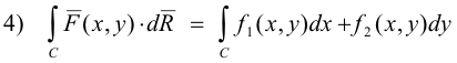
2] ∫_c F(x,y,z) ⋅ dR

where F(x, y, z) is a vector point function of x, y, z, R is a radius vector R(t) = x(t) i + y(t) j + z(t) k defining curve C, and the product is the dot product. This is the most common type of line integral.

3] ∫_c F(x,y,z) × dR

where F(x, y, z) is a vector point function of x, y, z, R is the radius vector R(t) = x(t) i + y(t) j + z(t) k defining curve C and the product is the cross product.

Our main interest is the line integral of type 2. When reference is made to line integrals, it is usually to Type 2 line integrals. We now define line integrals of Type 2 in terms of a limit of sums.

Def. Line integral. ∫_c F(x,y,z) ⋅ dR

where F(x, y, z) is a vector point function of x, y, z, R is the radius vector R(t) = x(t) i + y(t) j + z(t) k defining curve C, and the product is the dot product.

Let C be a rectifiable space curve (i.e. a curve of finite length) in xyz-space defined by parametric equations with parameter t on the closed interval [t = a, t = b] so that a point P on the curve has the position vector

R(t) = x(t)i + y(t)j + z(t)k .

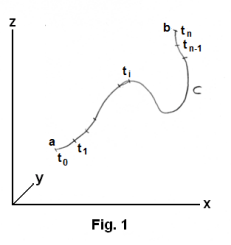
Let F be a vector point function defined and continuous at all points on interval [a, b] and let {a = t₀, t₁, ..., t_n= b} be a partition of interval [a, b]. Let τ_i be a point of the interval [t_{i -1}, t_i] and form the sum

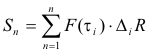
where

and the dot indicates the dot product. If this sum has a limit as the fineness of the partition approaches zero, the limit is the line integral of F over C, denoted by ∫_c F(t) ⋅ dR . If R is differentiable and F = Li + Mj + Nk, the line integral can be written as

If the parameter t represents the arc length s as measured from some start point, then the integral can be written as ∫_c F_t ds where F_t is the tangential component of F.

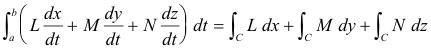
Integral ∫_cLdx + Mdy + Ndz .

Q. The integral ∫_CLdx + Mdy + Ndz is a line integral. What does it mean? Where does it come from? How do we understand it?

A. If F = Li + Mj + Nk and R = xi + yj + zk

∫_c F ⋅ dR = ∫_c( Li + Mj + Nk ) ⋅ (dxi + dyj + dzk) = ∫_CLdx + Mdy + Ndz

Some comments on line integrals. It is important to keep in mind that line integrals are different in a basic way from the ordinary integrals we are familiar with from elementary calculus. A line integral cannot be evaluated just as is. To evaluate it we need additional information — namely, the curve over which it is to be evaluated. This curve is generally given in parametric form such as

x = x(t)

y = y(t)

z = z(t) .

The integral is then altered when substituting in the parametric equivalents and is transformed into an ordinary integral in the variable t and is evaluated as any ordinary integral. There are some forms of line integrals that look a lot like ordinary integrals. For example,

could be either line integrals or ordinary integrals and we would have to know which they were from context. Also, the integral

looks a lot like an ordinary integral and we need to realize that it is a line integral and that we need to have a parametrically defined curve over which to integrate it. And realize that its appearance will change and its meaning become clearer after substituting in the parametric equivalents.

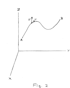
Application in physics. Line integrals of type ∫_cF ⋅ dR are of special interest in the field of physics. Let C be a space curve running from some point A to another point B in some region Q. Let C be defined by the position vector R(s) = x(s) i + y(s) j + z(s) k where s is the distance along the curve measured from point A. Let F(x, y, z) = f₁(x, y, z) i + f₂(x, y, z) j + f₃(x, y, z) k represent a force field defined over the region. Let T denote the unit tangent to the curve at point (x, y, z). Then F∙T is the component of F in the direction of the tangent T and the integral

∫_c F ⋅ T ds

represents the work done in moving a body from point A to point B along curve C. See Fig. 2. The unit vector T is equal to

T = dR/ds = dx/ds i + dy/ds j + dz/ds k

F∙T = (f₁ i + f₂ k + f₃ j)∙(dx/ds i + dy/ds j + dz/ds k )

= f₁(dx/ds) + f₂(dy/ds) + f₃(dz/ds)

and

Thus we can write

∫_cF ⋅ T ds = ∫_cF ⋅ dR

which is the form of 2] above.

From equation 3) above we state the following theorem:

Theorem 1. Let C be a space curve running from some point A to another point B in some region Q. Let curve C be defined by the radius vector R(s) = x(s) i + y(s) j + z(s) k where s is the distance along the curve measured from point A. Let F(x, y, z) = f₁(x, y, z) i + f₂(x, y, z) j + f₃(x, y, z) k represent a force field defined over the region. Let T denote the unit tangent to the curve at point (x, y, z). Then

∫_cF ⋅ T ds = ∫_cF ⋅ dR = ∫_c( f₁i + f₂j + f₃k ) ⋅ (dxi + dyj + dzk) = ∫_c f₁dx + f₂dy + f₃dz

represents the work done in moving an object along the curve from point A to point B.

Suppose now that we have a space curve C defined by the parametric equations

x = x(t)

y = y(t)

z = z(t),

or in vector form, R(t) = x(t) i + y(t) j + z(t) k , where t is time, and a force field defined by F(x, y, z) = f₁(x, y, z) i + f₂(x, y, z) j + f₃(x, y, z) k , in some region Q. We wish to compute the integral of

from point A to point B on curve C. If point A corresponds to time t = t₁ and point B corresponds to time t = t₂, then the integral becomes

where the primes denote derivatives with respect to t.

The line integral ∫_c f(x, y) dx in which the path of integration C is defined by a function g(x, y) = 0. Sometimes the path of integration C for a line integral in the xy plane

is defined by a function g(x, y) = 0, rather than parametrically by

x = g(t)

y = g(t) ,

giving rise to integrals of the type ∫_C f(x, y) dx to be evaluated.

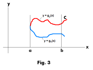
This integral ∫_C f(x, y) dx is then evaluated over an interval [a, b] of the x axis. The function f(x, y) is a scalar point function whose value varies with positions along the curve. To evaluate this integral it is necessary that the curve C is expressed as a single-valued function y = g(x) on the interval [a, b]. If the curve is like that shown in Fig. 3, it would have to be broken into two parts, one part expressed as y = g₁(x) [shown in blue in the figure] and the other expressed as y = g₂(x) [shown in red], and each part would have to be evaluated separately.

What is the quantity that this integral computes? Is there any intuitive meaning for it? If we subdivide the interval [a, b] into n equal parts and let x_i correspond to the midpoint of the i-th subdivision, the integral is given by

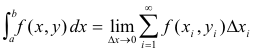
where the general term is f(x_i, y_i)Δx_i. What intuitive meaning does this quantity have (this general term)? Why would one be interested in computing a sum of these quantities? The answer: It is an abstract quantity that arises in different contexts.

Surface integrals.

************************

Let S be a surface and let f(P) be a point function defined on S. Divide S into a number of surface elements ΔS₁, ΔS₂, ... , ΔS_n of areas ΔA₁, ΔA₂, ... , ΔA_n. Let P_i be some point in the element ΔS_i. Then the surface integral of f over S is defined as

where the limit is taken as the maximum of the dimensions of the elements ΔS_i approaches zero.

If f(P) is expressed as a function F(x, y, z), where (x, y, z) are the coordinates of P, the surface integral becomes

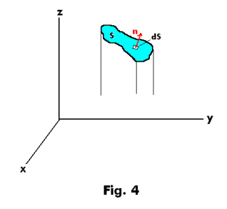
Unit normal, n. Let S be a two-sided surface such as the one shown in Fig. 4. Let one side of S be considered arbitrarily as the positive side (if S is a closed surface this is taken as the outer side). A unit normal n to any point of the positive side of S is called a positive or outward drawn normal.

Def. Vector dS = n dS. Let us associate with the differential of surface area dS a vector which we define as dS = n dS, whose magnitude is dS and whose direction is that of n.

Types of surface integrals. Let f be a scalar point function and A be a vector point function. The following are types of surface integrals:

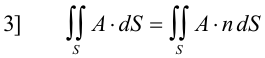
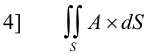
The integral of type 3 is of particular interest. It represents an integral of the flux A over a surface S.

To evaluate surface integrals we express them as double integrals taken over the projected area of the surface S on one of the coordinate planes. It is possible to do this if any line perpendicular to the coordinate plane chosen meets the surface in no more than one point. In general, this does not pose a problem since we can generally subdivide S into surfaces which do satisfy the restriction.

Volume integrals.

*************************

Consider a closed surface in space enclosing a volume V. Volume integrals can be defined in terms of limits of sums in the same way as was done with surface integrals above.

Let S be a closed surface enclosing a volume V. Let f(P) be a point function defined on V. Divide V into a number of volume elements ΔV₁, ΔV₂, ... , ΔV_n of volumes Δv₁, Δv₂, ... , Δv_n . Let P_i be some point in the element ΔV_i. Then the volume integral of f over V is defined as

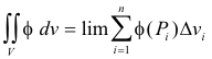
where the limit is taken as the maximum of the dimensions of the elements ΔVi approaches zero.

Types of volume integrals. Let f be a scalar point function and A be a vector point function. The following are types of volume integrals:

References.

Spiegel. Vector Analysis.

Hsu. Vector Analysis.

Wylie. Advanced Engineering Mathematics.

Taylor. Advanced Calculus.