Ways of viewing a non-singular linear transformation y = ax

There are different ways of viewing a non-singular linear transformation Y = AX.

1. As a change of basis. Y = AX can be viewed as a change of basis – a change to a basis whose basis vectors correspond to the columns of matrix A. In two and three dimensional space this corresponds to a change to a different coordinate system, a rotated coordinate system (the transformation Y = AX involves no translation).

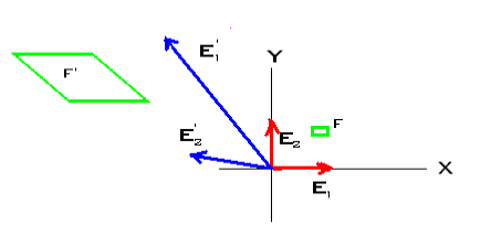
2. As a mapping of points of n-dimensional space into itself. We view the matrix A as an operator, a black box with an input and an output. You input a point and it outputs another point. In this way, matrix A maps the points of some figure in space into some other figure in space. A device for understanding how matrix A maps points is to observe what it maps its basis vectors, the elementary unit vectors , into. In fact, the elementary unit vectors will map into the column vectors of A. For example, consider the mapping

in 2-space. The elementary unit vector

maps into

 and the elementary unit vector

maps into

    .

We can then form an idea of what it would map something like a rectangle into. If it maps E₁ into E₁' and E₂ into E₂' then it will map the vector

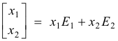
 into the vector E₁' + E₂' . See figure. Area F is mapped into area F’.

3. As a linear point transformation consisting of : 1) a change of basis to the eigenbasis of matrix A 2) a point transformation effected by a diagonal matrix in the eigenvector system 3) a change back to the original E-basis –- all represented by Y = BDB ^-1 X .

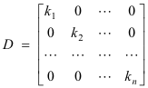
If the eigenvalues of A are distinct the linear transformation Y = AX can written as Y = BDB ^-1 X where D is a diagonal matrix whose diagonal elements consist of the eigenvalues of A and B is a matrix whose columns consist of the corresponding normalized eigenvectors of A. This representation of matrix A as equivalent to the product BDB ^-1 implies a three step sequence:

(1) A change of basis from the usual coordinate system (E-basis) to the Eigenvector Coordinate System (the canonical coordinate system where the actual point transformation is performed – and called the eigenbasis of A, a basis consisting of the eigenvectors of A).

(2) A linear point transformation effected by the diagonal matrix D in the Eigenvector Coordinate System. The effect of this transformation is simply stretching (or compressing) effects directed in the directions of the different coordinate system axes with magnitudes given by the eigenvalues.

(3) A change back to to the original E-basis.

4. As a linear point transformation consisting of : 1) a rotation in an orthonormal basis 2) a linear point transformation effected by a diagonal matrix consisting of stretching / compression in mutually orthogonal directions 3) another rotation in an orthonormal basis.

Let Y = AX be a non-singular linear transformation. Let be the n eigenvectors of the matrix (AA^T) ^-1 and B be a matrix whose columns consist of the corresponding normalized eigenvectors of (AA^T) ^-1 . Let

     .                                                                                            

Let

and

                                    C = A ^-1B D

Then A can be factored as:

                        A = BDC^T

Matrices B and C^T are both orthonormal matrices effecting “rotations” in n-dimensional space and matrix D effects stretching / compression in mutually orthogonal directions in n-space.